Chapter 14 Causal inference 2: Model-based estimation of causal parameters
Sources of inspiration when creating this practical: Luque Fernandez, M.A. et al. (2018) Stat Med 2018;37(16):2530-2546 and Smith et al. (2022) Stat Med 2022;41(2):407-432.
14.1 Introduction
In this exercise we learn to apply some R tools for estimating interesting causal parameters in the context of an observational study. The statistical methods to be introduced are (a) regression standardization or g-formula, (b) inverse probability weighting (IPW) with propensity scores and (c) double robust (DR) estimation combining approaches (a) and (b).
We illustrate these methods using simulated data. The exposure variable
\(X\) is binary (1/0) and the outcome variable \(Y\) is binary, too.
The interesting estimands are the causal risk difference (RD) and the
causal risk ratio (RR).
As a background story, we imagine a population of cancer patients, in whom the exposure, and four covariates \(Z = (Z_1, Z_2, Z_3, Z_4)\) plus the assumed marginal distributions of the latter are described in the table below:
| Variable | Description |
|---|---|
| \(X\) | treatment; 1: radiotherapy only, 0: radiotherapy + chemotherapy |
| \(Y\) | death during one year after diagnosis of cancer |
| \(Z_1\) | sex; 0: man, 1: woman; \(Z_1 \sim \text{Bern}(0.5)\) |
| \(Z_2\) | age group 0; young, 1: old; \(Z_2 \sim \text{Bern}(0.65)\) |
| \(Z_3\) | stage of cancer; 4 classes; \(Z_3 \sim \text{DiscUnif}(1, \dots, 4)\) |
| \(Z_4\) | comorbidity score; 5 classes; \(Z_3 \sim \text{DiscUnif}(1, \dots, 5)\) |
For simplicity, covariates \(Z_3\) and \(Z_4\) are treated as continuous variables with linear effects in the models.
- First, load the packages needed in this exercise
##
## Attaching package: 'Epi'
## The following object is masked from 'package:dagitty':
##
## paths- The assumed causal diagram is drawn using
dagittyand is shown below.
diagram <-
  dagitty("dag {
  Z2 -> Z3 -> Y
  Z2 -> Z4 -> Y
  Z2 -> Y
  Z2 -> Z3 -> X
  Z2 -> Z4 -> X
  Z2 -> X
  Z1 -> Z3 -> Y
  Z1 -> Z4 -> Y
  Z1 -> Y
  Z1 -> Z3 -> X
  Z1 -> Z4 -> X
}")

coordinates(diagram) <-
  list(
    x = c(X = 1, Y = 5, Z1 = 5, Z2 = 1, Z3 = 4, Z4 = 2),
    y = c(X = 2, Y = 2, Z1 = 0, Z2 = 0, Z3 = 1, Z4 = 1)
  )

plot(diagram)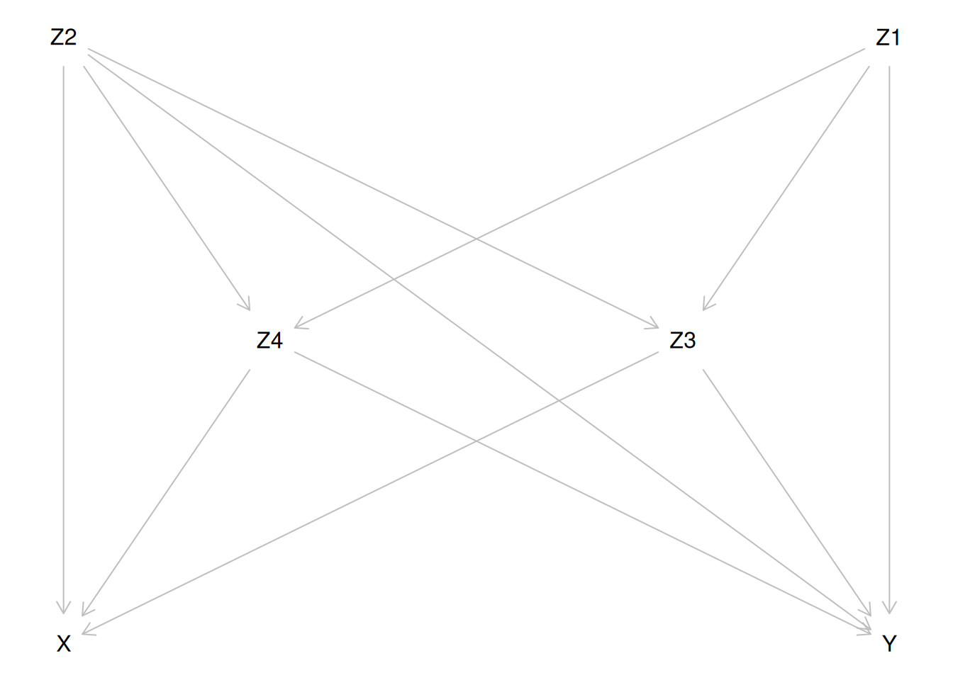
- For a more generic notation, the risk of death, i.e. the probability of \(Y=1\), will be expressed as the expected value of the binary outcome \(Y\), for instance \[ E(Y^{X=x}) = P(Y^{X=x}=1) \quad \text{and} \quad E(Y|X=x, Z=z) = P(Y=1|X=x, Z=z), \] where \(Z\) is the vector of relevant covariates.
The same principle is applied in expressing the conditional probability of being exposed, i.e. that of \(X=1\), given a set of covariate values \(Z=z\): \[ E(X|Z=z) = P(X=1|Z=z). \] The fitted and predicted probabilities of \(Y=1\) are denoted as \(\widehat{Y}\) and \(\widetilde{Y}\), respectively, with pertinent subscripts and/or superscripts.
Both \(X\) and \(Y\) are modelled by logistic regression. The expit-function
or inverse of the logit function is defined:
\(\text{expit}(u) = 1/(1 + e^{-u})\), \(u\in R\). This is equal to the
cumulative distribution function of the standard logistic distribution,
the values of which are returned in R by plogis(u). The R function
that returns values of the logit-function is qlogis().
The true exposure model for the dependence of exposure \(X\) on the covariates \(Z\) is specified as \[ E(X|Z_1 = z_1, \dots, Z_4 = z_4) = \text{expit}(-5 + 0.05z_2 + 0.25z_3 + 0.5z_4 + 0.4z_2z_4) . \] The assumed true outcome model \[ E(Y|X=x, Z_1 = z_1, \dots, Z_4 = z_4) = \text{expit}(-1 + x - 0.1z_1 + 0.35z_2 + 0.25z_3 + 0.20z_4 + 0.15z_2z_4) \] Note that \(X\) does not depend on \(Z_1\), and that in both models there is a product term \(Z_2 Z_4\), the effect of which appears weaker in the outcome model.
14.2 Control of confounding
Based on inspection of the causal diagram, can you provide justification for the claim that variables \(Z_2, Z_3\) and \(Z_4\) form a proper subset of the four covariates, which is sufficient to block all backdoor paths between \(X\) and \(Y\) and thus remove confounding?
Look what dagitty offers for sufficient sets:
## { Z2, Z3, Z4 }- Even though we have a sufficient set as claimed above, why it still might be useful to include covariate \(Z_1\), too, when modelling the outcome?
14.3 Generation of target population and true models
- Define two R-functions, which compute the expected values for the exposure and those for the outcome based on the assumed true exposure model and the true outcome model, respectively.
EX <- function(z2, z3, z4) {
  plogis(-5 + 0.05 * z2 + 0.25 * z3 + 0.5 * z4 + 0.4 * z2 * z4)
}
EY <- function(x, z1, z2, z3, z4) {
  plogis(-1 + x - 0.1 * z1 + 0.35 * z2 + 0.25 * z3 +
    0.20 * z4 + 0.15 * z2 * z4)
}- Define a function for generation of data by simulating random values from pertinent probability distributions based on the given assumptions.
genData <- function(N) {
  z1 <- rbinom(N, size = 1, prob = 0.5) # Bern(0.5)
  z2 <- rbinom(N, size = 1, prob = 0.65) # Bern(0.65)
  z3 <- trunc(runif(N, min = 1, max = 5), digits = 0) # DiscUnif(1,4)
  z4 <- trunc(runif(N, min = 1, max = 6), digits = 0) # DiscUnif(1,5)
  x <- rbinom(N, size = 1, prob = EX(z2, z3, z4))
  y <- rbinom(N, size = 1, prob = EY(x, z1, z2, z3, z4))
  data.frame(z1, z2, z3, z4, x, y)
}- Generate a data frame
popfor a big target population of 1000000 subjects
14.4 Factual and counterfactual risks - associational and causal contrasts
- Compute the factual risks of death for the two exposure groups
\[ E(Y|X=x) = P(Y=1|X=x) = \frac{P(Y=1\ \&\ X=x)}{P(X=x)},
\quad x=0,1, \]
in the whole target population, as well as their
associational contrasts: risk difference, risk ratio, and odds
ratio. Before that let us define a useful function
Contr():
Contr <- function(mu1, mu0) {
  RD <- mu1 - mu0
  RR <- mu1 / mu0
  OR <- (mu1 / (1 - mu1)) / (mu0 / (1 - mu0))
  return(c(Risk1=mu1, Risk0=mu0, RD = RD, RR = RR, OR = OR))
}
Ey1fact <- with(pop, sum(y == 1 & x == 1) / sum(x == 1))
Ey0fact <- with(pop, sum(y == 1 & x == 0) / sum(x == 0))
round(Contr(Ey1fact, Ey0fact), 4)
## Risk1 Risk0 RD RR OR
## 0.8955 0.6280 0.2674 1.4258 5.0735The one-year mortality is quite high in both groups. – How much bigger is the risk of death of those factually exposed to radiotherapy only as compared with those receiving chemotherapy, too?
Comment: With such a high baseline probability of the outcome the risk ratio cannot become greater than 1/0.628 = 1.59. For relative comparisons one could also consider using survival ratio (SR) For instance, here the associational survival ratio is \[ \text{SR} = (1-0.8955)/(1-0.6280) = 0.1045/0.372 = 0.2809 = 1/3.56 . \] See also Huitfeldt et al. (2022) “Shall we count the living or the dead?’’ for discussion concerning the choice between risk ratio and survival ratio for a relative effect measure.
- Compute now the true counterfactual or potential risks of death \[ E(Y_i^{X_i=x}) = P(Y_i^{X_i=x}=1) = \pi_i^{X_i=x} \] for each individual under the alternative treatments or exposure values \(x=0,1\) with given covariate values. After that derive the average or overall counterfactual risks \(E(Y^{X=1}) = \pi^1\) and \(E(Y^{X=0}) = \pi^0\) in the population, and finally the true marginal causal contrasts describing the effect of \(X\): \[\begin{aligned} \text{RD} & = E(Y^{X=1})-E(Y^{X=0}), \qquad \text{RR} = E(Y^{X=1})/E(Y^{X=0}), \\ \text{OR} & = \frac{E(Y^{X=1})/[1 - E(Y^{X=1})]}{E(Y^{X=0})/[1 - E(Y^{X=0})] } \end{aligned} \]
pop <- transform(pop,
  EY1.ind = EY(x = 1, z1, z2, z3, z4),
  EY0.ind = EY(x = 0, z1, z2, z3, z4)
)
EY1pot <- mean(pop$EY1.ind)
EY0pot <- mean(pop$EY0.ind)
round(Contr(EY1pot, EY0pot), 4)
## Risk1 Risk0 RD RR OR
## 0.8274 0.6531 0.1743 1.2668 2.5455See Colnet et al. (2023) for a thorough comparison of the different causal contrasts. Among these, RD appears to have more favourable mathematical properties than RR and OR, and in several respects OR is a particularly problematic measure of causal effect.
Compare the associational contrasts (e.g. RD=0.2674) computed in item 1 with the causal contrasts here. What do you conclude about the amount of confounding bias in the associational contrasts?
To illustrate what happens in a realistic setting involving some random variability we shall draw a random sample of 5000 patients using systematic sampling. We also compute the estimates of the counterfactual quantities from this sample based on the true models.
## 'data.frame':    5000 obs. of  8 variables:
##  $ z1     : int  0 0 1 1 1 1 1 1 0 0 ...
##  $ z2     : int  1 1 1 1 1 0 1 1 0 1 ...
##  $ z3     : num  4 1 1 4 4 4 3 1 1 4 ...
##  $ z4     : num  1 2 2 3 2 1 5 3 3 3 ...
##  $ x      : int  0 0 0 1 0 0 1 0 1 0 ...
##  $ y      : int  0 0 0 1 0 1 1 1 1 0 ...
##  $ EY1.ind: num  0.846 0.786 0.769 0.909 0.875 ...
##  $ EY0.ind: num  0.668 0.574 0.55 0.786 0.721 ...
EY1pot.samp <- mean(samp$EY1.ind)
EY0pot.samp <- mean(samp$EY0.ind)
round(Contr(EY1pot.samp, EY0pot.samp), 4)## Risk1 Risk0 RD RR OR
## 0.8257 0.6500 0.1757 1.2704 2.5514The sample estimates of the counterfactual risks and their contrasts based on the true models seem to be not too far from the true values of those estimands.
- Some perspective to the random variability in the estimation of parameters of interest is provided by the numbers of cases and non-casses in the two exposure groups of the sample
stat.table(index=list("Outcome"=factor(y), "Exposure"=factor(x)),
           contents=list(count(), percent(y)),
           margins=TRUE, data=samp  )
## ----------------------------------
## --------Exposure---------
## Outcome 0 1 Total
## ----------------------------------
## 0 1519 81 1600
## 36.3 10.0 32.0
##
## 1 2668 732 3400
## 63.7 90.0 68.0
##
##
## Total 4187 813 5000
## 100.0 100.0 100.0
## ----------------------------------The group sizes are very different; only 16 % of the patients were exposed to radiotherapy only.
The statistical precision in any comparison between the exposure groups based on the sample data is very much dominated by the smallest count in this fourfold table, i.e. the number of non-cases among the exposed, which is not very big.
14.5 Outcome modelling and estimation of causal contrasts by g-formula
As the first approach for estimating causal contrasts of interest we apply the method of regression standardization or g-formula. It is based on a hopefully realistic enough model for \(E(Y|X=x, Z=z)\), i.e. how the risk of the outcome is expected to depend on the exposure variable \(X\) and on a sufficient set \(Z\) of confounders. The potential or counterfactual risks \(E(Y^{X=x}), x=0,1\), are marginal expectations of the above quantities, standardized over the joint distribution of the confounders \(Z\) in the target population. \[ E(Y^{X=x}) = E_Z[E(Y|X=x,Z)] = \sum_z P(Y=1|X=x, Z=z)P(Z=z), \quad x=0,1, \] in which \(E_Z[\dots]\) is a general expression for the marginal expectation and \(\sum_z \dots\) provides the formula for the special case of a binary outcome \(Y\) and a categorical covariate \(Z\).
- Assume now a slightly misspecified model
mYfor the outcome, which contains only the main effect terms of the explanatory variables: \[ \pi_i = E(Y_i|X_i=x_i, Z_{i1}=z_{i1}, \dots, Z_{i4}=z_{i4}) = \text{expit}\left(\beta_0 + \delta x_i + \sum_{j=1}^4 \beta_j z_{ij} \right) . \] Fit this model on the data of the whole target population using functionglm()
mY <- glm(y ~ x + z1 + z2 + z3 + z4, family = binomial, data = pop)
round(ci.lin(mY, Exp = TRUE)[, c(1, 5:7)], 4)
## Estimate exp(Est.) 2.5% 97.5%
## (Intercept) -1.2545 0.2852 0.2806 0.2900
## x 1.0560 2.8750 2.8267 2.9240
## z1 -0.1012 0.9038 0.8958 0.9118
## z2 0.7592 2.1366 2.1170 2.1563
## z3 0.2525 1.2872 1.2821 1.2924
## z4 0.2838 1.3282 1.3238 1.3327The point estimates for the intercept, \(X, Z_1\) and \(Z_3\) seem to be reasonably close to the given parameter values in the true model, but those of \(Z_2\) and \(Z_4\) are different. This is because the fitted model ignored the product term \(Z_2 Z_4\).
- For each subject \(i\), compute the fitted individual risk
\(\widehat{Y_i}\) saved into variable
yh(actually these will not be needed until the end of this practical!) as well as the predicted potential (counterfactual) risks \(\widetilde{Y_i}^{X_i=x}\) saved intoyp1andyp0for exposure levels \(x=0,1\), respectively, keeping the individual values of the \(Z\)-variables as they are in the observed data.
pop$yh <- predict(mY, type = "response")  #  fitted risk
pop$yp1 <- predict(mY, newdata = data.frame(
  x = rep(1, N),      # predicted risk assuming x=1, i.e. "if exposed"
  pop[, c("z1", "z2", "z3", "z4")]
), type = "response")
pop$yp0 <- predict(mY, newdata = data.frame(
  x = rep(0, N),      # predicted risk assuming x=0, i.e. "if unexposed"
  pop[, c("z1", "z2", "z3", "z4")]
), type = "response")- Applying the method of standardization or g-formula we now compute
the point estimates \[ \widehat{E}_g(Y^{X=x}) =
\frac{1}{n} \sum_{i=1}^n \widetilde{Y}_i^{X_i=x}, \quad x=0,1. \]
of the two counterfactual risks \(E(Y^{X=1}) = \pi^1\) and
\(E(Y^{X=0})=\pi^0\) as well as
those of the marginal causal contrasts.
##  Risk1  Risk0     RD     RR     OR
## 0.8331 0.6503 0.1828 1.2811 2.6837Comment: The joint distribution of the confounders \(Z\) in the target population is here manifested in the actual distribution of the data in that population. Thus, marginal expectations \(E_Z[E(X=x, Z)]\) are obtained by simple computation of the arithmetic means of the individually predicted values \(\widetilde{Y_i}^{X_i=x}\) of the outcome for the two exposure levels in this population.
Compare the estimated contrasts with those obtained from applying the true model (RD = 0.1743) in item 4.4 above. How big is the bias due to misspecification of the outcome model?
Compare in particular the estimate of the marginal OR here with the conditional OR obtained in item 5.1 from the pertinent coefficient in the logistic model. Which one is closer to 1?
- Perform the same calculations using the tools in package
stdReg2but now on the sample data. (see Sjölander 2016 and Sachs et al 2025). Using functionstandardize_glm()the same logistic model is fitted, and the point estimates together with the confidence intervals for the causal risk difference and causal risk ratio are computed. The results are saved into a list, for which we give the namemY.std.
The main results are shown in four small windows
after applying the print method on mY.std
mY.std <- standardize_glm(
 formula = y ~ x + z1 + z2 + z3 + z4,
 family = "binomial",
 data = samp,
 values = list(x = 0:1),
 contrasts = c("difference", "ratio"),
 reference = 0
)
mY.std
## Outcome formula: y ~ x + z1 + z2 + z3 + z4
## Outcome family: quasibinomial
## Outcome link function: logit
## Exposure: x
##
## Tables:
## x Estimate Std.Error lower.0.95 upper.0.95
## 1 0 0.656 0.00731 0.641 0.670
## 2 1 0.849 0.01533 0.819 0.879
##
## Reference level: x = 0
## Contrast: difference
## x Estimate Std.Error lower.0.95 upper.0.95
## 1 0 0.000 0.0000 0.000 0.000
## 2 1 0.193 0.0172 0.159 0.227
##
## Reference level: x = 0
## Contrast: ratio
## x Estimate Std.Error lower.0.95 upper.0.95
## 1 0 1.00 0.0000 1.00 1.00
## 2 1 1.29 0.0278 1.24 1.35The point estimates seem to be well within a resonable error margin when
compared to those, which you got by explicit computations for the whole
population data (e.g. RD=0.1828) in the previous item. (You could also
run standardize_glm() with data=pop to convince yourself that
stdReg2 indeed provides the same point estimates as obtained above
for the whole population from modelmY).
In stdReg2, the standard errors are obtained by the multivariate delta
method built upon M-estimation (Stefanski & Boos
2002) and robust sandwich
estimator of the pertinent covariance matrix. Approximate confidence
intervals are derived from these in the usual way.
14.6 Inverse probability weighting (IPW) by propensity scores
Our next method is based on weighting each individual observation by the inverse of the probability of belonging to that particular exposure group, which was realized, this probability being predicted by the determinants of exposure.
- First, we examine the validity of this approach by fitting the true
model on the whole population data.
To repeat, the model is \[ p_i = E(X_i| Z_{1i} = z_{1i}, \dots, Z_{4i} = z_{4i}) = \text{expit}(\gamma_0 + \gamma_2 z_{2i} + \gamma_3 z_{i3} + \gamma_4 z_{4i} + \gamma_{24} z_{2i}z_{4i}), \quad i=1, \dots N \]
mX <- glm(x ~ z2 + z3 + z4 + z2:z4,
  family = binomial(link = logit), data = pop)
round(ci.lin(mX, Exp = TRUE)[, c(1, 5)], 4)
## Estimate exp(Est.)
## (Intercept) -5.0196 0.0066
## z2 0.0825 1.0860
## z3 0.2474 1.2807
## z4 0.5035 1.6544
## z2:z4 0.3956 1.4852The estimated coefficients and ORs are quite close to the true values as given in the introduction section.
- From the fitted model we then extract the propensity scores, i.e. fitted probabilities of belonging to exposure group 1: \(\text{PS}_i = \widehat{p_i}\). We also make a simple comparison of the distribution of the scores between the two groups by common summary measures.
## $`0`
##    Min. 1st Qu.  Median    Mean 3rd Qu.    Max.
## 0.01381 0.03660 0.07509 0.13568 0.18053 0.63357
##
## $`1`
##    Min. 1st Qu.  Median    Mean 3rd Qu.    Max.
## 0.01381 0.18053 0.35460 0.35172 0.51319 0.63357
How different are the distributions? Can one judge from these summaries, that they are sufficiently overlapping?
Informative graphical tools for examining overlap and covariate balance
are contained in package PSweight,
and they are introduced in the next section.
- We then compute the inverse probability weights (IPW), also known as inverse probability treatment weights (IPTW): \[\begin{aligned} W_i & = \frac{1}{\text{PS}_i}, \quad \text{when }\ X_i=1, \\ W_i & = \frac{1}{1-\text{PS}_i}, \quad \text{when }\ X_i=0 . \end{aligned} \] Look at the sum as well as the distribution summary of the weights in the exposure groups. In an ideal situation with a well-specified exposure model the sum of weights should be close to to the population size in both groups.
##         0         1
## 999884.4 1001553.5- Compute now the weighted estimates of the potential or counterfactual risks for both exposure categories \[ \widehat{E}_w(Y^{X = x}) = \frac{ \sum_{i=1}^n {\mathbf 1}_{ \{X_i=x\} } W_i Y_i } {\sum_{i=1}^n {\mathbf 1}_{ \{X_i=x\} }W_i} = \frac{ \sum_{X_i = x} W_i Y_i }{\sum_{X_i=x} W_i}, \quad x = 0,1, \] and their causal contrasts, for instance \[ \widehat{\text{RD}}_{w} = \widehat{E}_w(Y^{X = 1}) - \widehat{E}_w(Y^{X = 0}) = \frac{ \sum_{i=1}^n X_i W_i Y_i }{\sum_{i=1}^n X_i W_i} - \frac{ \sum_{i=1}^n (1-X_i) W_i Y_i }{\sum_{i=1}^n (1-X_i) W_i}\]
EY1pot.w <- sum(pop$x * pop$w * pop$y) / sum(pop$x * pop$w)
EY0pot.w <- sum((1 - pop$x) * pop$w * pop$y) / sum((1 - pop$x) * pop$w)
round(Contr(EY1pot.w, EY0pot.w), 4)
## Risk1 Risk0 RD RR OR
## 0.8260 0.6522 0.1737 1.2664 2.5304These results seem to be practically equal to the true values (e.g. true RD=0.1743).
Comment: If you apply the package PSweight introduced in the next
section but
use the whole population data, i.e. putting data=pop, you would see
that the estimates of the causal contrasts would be the same as obtained
here.
14.7 IPW estimation using R package PSweight
We shall now try IPW-estimation with a misspecified model, such that we
include all \(Z\)-variables but none of their pairwise interactions. We do
this on the sample data only. In computations we utilize the R package
PSweight
(see PSweight vignette).
- The exposure model is fitted using
glm(), and the weights are obtained using functionSumStat()in packagePSweight:
mX2 <- glm(x ~ z1 + z2 + z3 + z4, family = binomial, data = samp)
round(ci.lin(mX2, Exp = TRUE)[, c(1:2, 5:7)], 3)
## Estimate StdErr exp(Est.) 2.5% 97.5%
## (Intercept) -6.520 0.229 0.001 0.001 0.002
## z1 0.115 0.086 1.121 0.948 1.327
## z2 1.722 0.116 5.594 4.460 7.017
## z3 0.227 0.038 1.255 1.164 1.353
## z4 0.855 0.038 2.351 2.183 2.531Note that apart from weights IPW for the whole population, other kinds
of weights can also be computed. These are relevant when estimating
other types of causal contrasts, like “average treatment effect among
the treated” (ATT, see below) and “average treatment effect in the
overlap (or equipoise) population” (ATO).
PSweightincludes some useful tools to examine the properties of the distribution of the propensity scores. First we draw density plots showing, how well the distributions of propensity scores (and 1 - PS, too) are overlapping between the exposure groups – NB. You may get a warning about usage of aggplot2aesthetic in the density plot implemented inPSweight, this feature being now outdated in the newest version ofggplot2. Nonetheless, the density plot will after all be drawn, if you go down on the Console window and “Press [enter] to continue”!
## Warning: Using `size` aesthetic for lines was deprecated in ggplot2 3.4.0.
## ℹ Please use `linewidth` instead.
## ℹ The deprecated feature was likely used in the PSweight package.
##   Please report the issue to the authors.
## This warning is displayed once per session.
## Call `lifecycle::last_lifecycle_warnings()` to see where this warning was
## generated.
## Propensity score for group 0## Press [enter] to continue## Propensity score for group 1Are the distributions of the propensity scores very different?
- We then create a diagnostic plot to examine the covariate balance between the groups:
In this plot, it would be desirable that the horisontal values of the standardized mean differences for a given type of weights are less than 0.1. – There seems to be some issue with the balance with regard to the estimation of our target parameters based on this exposure model.
- Estimation and reporting of the causal contrasts: Weights must be
IPWwhen estimating the causal effect generalized to the whole target population. For relative contrasts, the summary method provides the results on the log-scale; therefore exp-transformation.
## Original group value:  0, 1
##
## Point estimate:
## 0.6565, 0.8027##
## Closed-form inference:
##
## Original group value: 0, 1
##
## Contrast:
## 0 1
## Contrast 1 -1 1
##
## Estimate Std.Error lwr upr Pr(>|z|)
## Contrast 1 0.146179 0.036149 0.075329 0.21703 5.259e-05 ***
## ---
## Signif. codes: 0 '***' 0.001 '**' 0.01 '*' 0.05 '.' 0.1 ' ' 1##
## Closed-form inference:
##
## Inference in log scale:
## Original group value: 0, 1
##
## Contrast:
## 0 1
## Contrast 1 -1 1
##
## Estimate Std.Error lwr upr Pr(>|z|)
## Contrast 1 0.20103 0.04547 0.11191 0.29015 9.816e-06 ***
## ---
## Signif. codes: 0 '***' 0.001 '**' 0.01 '*' 0.05 '.' 0.1 ' ' 1## [1] 1.223 1.118 1.337## [1] 2.128 1.367 3.315Comparing these with the previous IPW estimates (e.g. RD=0.1737) as well as the true values (RD=0.1743), there perhaps can be seen indication of some bias due to misspecification. Remember, though, that these estimates are from the sample data with relatively wide error margins.
The standard errors provided by PSweight are by default based on the
empirical sandwich covariance matrix and application of delta method as
appropriate. Bootstrapping is also possible but is computationally very
intensive and is recommended to be used only in relatively small
samples.
14.8 Effect of exposure among those exposed
If we are interested in the causal contrasts describing the effect of exposure among those exposed (like ATE), the relevant factual and counterfactual risks in that subset are conditional on being exposed:
\[\begin{aligned} \pi^1_1 & = E(Y^{X=1}|X=1) = E(Y|X=1) = \pi_1, \\ \pi^0_1 & = E(Y^{X=0}|X=1) = \sum_{X_i=1} E(Y|X=0, Z=z)P(Z=z|X=1) \end{aligned}\]
We are thus making and “observed vs. expected” comparison, in which the \(z\)-specific risks in the unexposed are weighted by the distribution of \(Z\) in the exposed subset of the target population.
- We shall first estimate these \(z\)-specific “observed” or factual and
“expected” or counterfactual risks and their contrasts conditional
on being exposed from the slightly misspecified outcome model
mYfitted on the whole population data:
EY1att.g <- mean(subset(pop, x == 1)$yp1)
EY0att.g <- mean(subset(pop, x == 1)$yp0)
round(Contr(EY1att.g, EY0att.g), 4)
## Risk1 Risk0 RD RR OR
## 0.8955 0.7565 0.1389 1.1836 2.7568Compare the results here with those (e.g. RD=0.1828) meant to describe
the overall causal contrasts among the whole target population from the
same model mY. What do you observe?
What is your guess about the causal effect of exposure among the unexposed; is it bigger or smaller than it is among the exposed or among the whole population?
Incidentally, the true causal contrasts among the exposed based on the true model are similarly obtained from the quantities in item 4.2 above:
EY1att <- mean(subset(pop, x == 1)$EY1.ind)
EY0att <- mean(subset(pop, x == 1)$EY0.ind)
round(Contr(EY1att, EY0att), 4)
## Risk1 Risk0 RD RR OR
## 0.8957 0.7684 0.1273 1.1657 2.5886Compare the estimates in the previous item (e.g. RD\(_1\) = 0.1389) with the true values obtained here. The misspecification of the outcome model implies some bias in these results, too.
- When wishing to estimate the effect of exposure among the exposed
using the IPW approach, then the weights are \(W_i = 1\) for the
exposed and \(W_i = \text{PS}_i/(1-\text{PS}_i)\) for the unexposed.
We shall again use
PSweightwith sample data but with another choice of weights:
## Original group value:  0, 1
## Treatment group value:  1
##
## Point estimate:
## 0.7579, 0.9004## Estimate Std.Error z value lwr upr Pr(>|z|)
## Contrast 1 0.1424 0.0147 9.6623 0.1135 0.1713 0## Estimate Std.Error z value lwr upr Pr(>|z|)
## Contrast 1 1.188 1.018 13678.08 1.147 1.231 1Compare the results here with those obtained by g-formula in item 8.1 and with the true contrasts above.
14.9 Double robust (DR) estimation
We may try to reduce the bias in the estimation of the target parameters, which would be caused by possible specification error either in the outcome model or in the exposure model using some double robust (DR) approach. These methods combine the principle of regression standardization with that of IPW/propensity scores.
A classical DR method is augmented IPW estimation (AIPW), in which the estimator can be expressed in two alternative ways: either a regression-standardized estimator corrected by IPW, or an IPW-estimator corrected by standardization.
\[\begin{aligned} \widehat{E}_a(Y^{X=x}) & = \widehat{E}_g(Y^{X=x}) + \frac{1}{n} \sum_{i=1}^n {\mathbf 1}_{\{X_i=x\}} W_i ( Y_i - \widetilde{Y}_i^{X_i=x} ) \\ & = \widehat{E}_w(Y^{X=x}) + \frac{1}{n} \sum_{i=1}^n ( 1 - {\mathbf 1}_{\{X_i=x\}} W_i ) \widetilde{Y}_i^{X_i=x}. \end{aligned}\]
- We apply the AIPW method first in the whole population by direct
combination of the results that we obtained from the slightly
misspecified outcome model
mYwith those from the well-specified exposure modelmX.
EY1pot.a <- EY1pot.g + mean( 1*(pop$x==1) * pop$w * (pop$y - pop$yp1) )
EY0pot.a <- EY0pot.g + mean( 1*(pop$x==0) * pop$w * (pop$y - pop$yp0) )
round(Contr(EY1pot.a, EY0pot.a), 4)
## Risk1 Risk0 RD RR OR
## 0.8259 0.6523 0.1737 1.2663 2.5296Compare these results with those obtained by g-formula (e.g. RD=0.1828) and by the IPW method (RD=0.1737) as well as with the true values (RD = 0.1743) of the parameters. – Was correction of the g-estimates by IPW successful?
- AIPW-estimates and confidence intervals for the causal contrasts of
interest can be obtained, for instance, using
PSweight. We will assign the outcome modelmYinto the argumentout.formula. We again combine this slightly misspecified outcome model with the correct exposure modelmXand perform the estimation on the sample data.
aipw.psw <- PSweight(ps.formula = mX, out.formula = mY, yname = "y",
                     data = samp, weight = "IPW")
aipw.psw
## Original group value: 0, 1
##
## Point estimate:
## 0.6576, 0.8234## Estimate Std.Error z value lwr upr Pr(>|z|)
## Contrast 1 0.1658 0.0262 6.3406 0.1146 0.2171 0## Estimate Std.Error z value lwr upr Pr(>|z|)
## Contrast 1 1.252 1.033 1024.995 1.175 1.334 1The estimates here are quite close to the true values, but the error margins are still relatively wide.
- Alternatively,
stdReg2can also be utilized for double-robust estimation of causal contrasts. It leans, though, on a somewhat different approach. The method developed for the types of outcomes and models covered by generalized linear models (GLM) is known by its initialism IPTW GLM. It is based on weighted maximum likelihood fitting of the outcome model. The weights are inverses of the propensity scores obtained from the pertinent exposure model. Computation of standard errors and confidence intervals uses the influence function approach, which among other things takes into account the fact that weighting is based on estimated propensity scores. – See Gabriel et al 2024 for details of IPTW GLM.
We shall try this method for the sample data with the script below:
dr.std <- standardize_glm_dr(
          formula_outcome = y ~ x + z1 + z2 + z3 + z4,
          formula_exposure = x ~ z2 + z3 + z4 + z2:z4,
          data = samp,
          family_outcome = "binomial",
          family_exposure = "binomial",
          values = list(x = 0:1),
          contrasts = c("difference", "ratio"), reference = 0)
dr.std
## Doubly robust estimator with:
##
## Exposure formula: x ~ z2 + z3 + z4 + z2:z4
## Exposure link function: logit
## Outcome formula: y ~ x + z1 + z2 + z3 + z4
## Outcome family: quasibinomial
## Outcome link function: logit
## Exposure: x
##
## Tables:
## x Estimate Std.Error lower.0.95 upper.0.95
## 1 0 0.658 0.00732 0.643 0.672
## 2 1 0.827 0.02500 0.778 0.876
##
## Reference level: x = 0
## Contrast: difference
## x Estimate Std.Error lower.0.95 upper.0.95
## 1 0 0.000 0.000 0.000 0.00
## 2 1 0.169 0.026 0.119 0.22
##
## Reference level: x = 0
## Contrast: ratio
## x Estimate Std.Error lower.0.95 upper.0.95
## 1 0 1.00 0.0000 1.00 1.00
## 2 1 1.26 0.0404 1.18 1.34The point estimates are not much different from those obtained above when applying AIPW estimation.
14.10 DR estimation with flexible learning algorithms
It may not be easy to specify a conventional generalized linear models or even a generalized additive model for exposure and outcome, which would be sufficiently realistic, but not suffering from overfitting. Modern approaches of statistical learning, a.k.a. “machine learning” provide tools for flexible modelling, which may be used to reduce the risk of misspecification, if thoughtfully applied.
There are a few R packages in which some general algorithmic approaches
for supervised learning are implemented for estimating causal
parameters. For instance, package AIPW (see Zhong et al.,
2021) utilizes several learning
algorithms for exposure and outcome modelling and then performs AIPW
estimation of the parameters of interest coupled with calculation of
confidence intervals. Package tmle (see Karim and Frank,
2021) performs same tasks but
uses the targeted maximum likelihood estimation (TMLE) approach in
estimation.
Both AIPW and tmle lean on the SuperLearner package, which uses
multiple learning algorithms (e.g. GLM, GAM, Random Forest, Recursive
Partitioning, Gradient Boosting, etc.) for constructing predictions of
the counterfactual quantities, and then creates an optimal weighted
average of those models, a.k.a. an “ensemble”. These algorithms are
computationally highly intensive. Fitting models with only 3 or 4
covariates as in this practical for our whole target cohort of 1,000,000
subjects would take hours on an ordinary laptop. With a sample of 5000
it woul still take several minutes.
14.11 Extra: Computations in the TMLE method
Finally, a few words on, how causal contrasts are estimated using the
TMLE, when we have fitted an outcome model, like mY, and an exposure
model, like mX. TMLE corrects the estimates obtained from the outcome
model by some elements derived from the exposure model. The correction,
though, is not as intuitive and transparent as it is in AIPW. See
Schuler and Rose (2017) for more
details.
We show the steps of computation using the data covering the whole target population.
- In the first step we utilize the propensity scores previously
obtained from fitting the correct exposure model and compute from
them the “clever covariates”
H1andH0:
- Then, a working model is fitted for the outcome, in which the
clever covariates are explanatory variables, but the model also
includes as an offset term the previously fitted linear predictor
from the original outcome model
mY: \(\widehat{\eta}_i = \text{logit}(\widehat Y_i)\) based on the observed exposure \(X_i=x\) for each subject \(i\), where the fitted values \(\widehat Y_i\) were saved into vectoryhalready in item 5.2 above. Moreover, the intercept is removed from the model.
epsmod <- glm(y ~ -1 + H0 + H1 + offset(qlogis(yh)),
  family = binomial(link = logit), data = pop)
eps <- coef(epsmod)
eps
## H0 H1
## 0.007655093 -0.002475541- The logit-transformed predicted values \(\widetilde{Y}_i^{X_i=1}\) and
\(\widetilde{Y}_i^{X_i=0}\) of the potential or counterfactual
individual risks from the original outcome model
mYare now corrected by the estimated coefficients of the clever covariates, and the corrected predictions are returned to the original probability scale.
pop$ypred0.H <- plogis(qlogis(pop$yp0) + eps[1] / (1 - pop$PS))
pop$ypred1.H <- plogis(qlogis(pop$yp1) + eps[2] / pop$PS)- Estimates of the causal contrasts are obtained as before
##  Risk1  Risk0     RD     RR     OR
## 0.8260 0.6523 0.1737 1.2663 2.5301
These are similar to previous results obtained by AIPW when computed for the whole population with the correct exposure model, and they are very close to the true values (e.g. RD=0.1743), too.