Chapter 9 Causal inference
9.1 Proper adjustment for confounding in regression models
The first exercise of this session will ask you to simulate some data according to pre-specified causal structure (don’t take the particular example too seriously) and see how you should adjust the analysis to obtain correct estimates of the causal effects.
Suppose one is interested in the effect of beer-drinking on body weight. Let’s assume that in addition to the potential effect of beer on weight, the following is true in reality:
- Men drink more beer than women
- Men have higher body weight than women
- People with higher body weight tend to have higher blood pressure
- Beer-drinking increases blood pressure
The task is to simulate a dataset in accordance with this model, and subsequently analyse it to see, whether the results would allow us to conclude the true association structure.
- Sketch a DAG (not necessarily with R) to see, how should one generate the data
- Suppose the actual effect sizes are following:
- The probability of beer-drinking is 0.2 for females and 0.7 for males
- Men weigh on average \(10kg\) more than women.
- One kg difference in body weight corresponds in average to \(0.5mmHg\) difference in (systolic) blood pressures.
- Beer-drinking increases blood pressure by \(10mmHg\) in average.
- Beer-drinking has no effect on body weight.
The R commands to generate the data are:
set.seed(23957)
bdat <- data.frame(sex = c(rep(0, 500), rep(1, 500)))
# a data frame with 500 females, 500 males
bdat$beer <- rbinom(1000, 1, 0.2 + 0.5 * bdat$sex)
bdat$weight <- 60 + 10 * bdat$sex + rnorm(1000, 0, 7)
bdat$bp <-
110 + 0.5 * bdat$weight + 10 * bdat$beer + rnorm(1000, 0, 10)- Now fit the following models for body weight as dependent variable and beer-drinking as independent variable. Look, what is the estimated effect size
- Unadjusted (just simple linear regression)
- Adjusted for sex
- Adjusted for sex and blood pressure
library(Epi)
m1a <- lm(weight ~ beer, data = bdat)
m2a <- lm(weight ~ beer + sex, data = bdat)
m3a <- lm(weight ~ beer + sex + bp, data = bdat)
ci.lin(m1a)
## Estimate StdErr z P 2.5% 97.5%
## (Intercept) 62.269170 0.3470984 179.39919 0.000000e+00 61.588870 62.949470
## beer 5.296786 0.5256653 10.07635 7.029082e-24 4.266501 6.327072## Estimate StdErr z P 2.5% 97.5%
## (Intercept) 59.4647612 0.3248236 183.0678546 0.000000e+00 58.828119 60.1014038
## beer -0.1263823 0.5198915 -0.2430936 8.079329e-01 -1.145351 0.8925863
## sex 10.3378209 0.5156149 20.0494980 2.038922e-89 9.327234 11.3484076## Estimate StdErr z P 2.5% 97.5%
## (Intercept) 26.9076970 2.82806033 9.514541 1.825162e-21 21.3648006 32.4505934
## beer -2.5165947 0.53015283 -4.746923 2.065344e-06 -3.5556752 -1.4775143
## sex 9.1700486 0.49469045 18.536943 1.039662e-76 8.2004732 10.1396241
## bp 0.2327287 0.02009792 11.579736 5.220635e-31 0.1933374 0.2721199- What would be the conclusions on the effect of beer on weight, based on the three models? Do they agree? Which (if any) of the models gives an unbiased estimate of the actual causal effect of interest?
Solution. (Note - for the estimated coefficient of beer, 0 should be included in the confidence interval - there is just one model where that is true)
How can the answer be seen from the graph?
Now change the data-generation algorithm so, that in fact beer-drinking does increase the body weight by 2kg. Look, what are the conclusions in the above models now. Thus the data is generated as before, but the weight variable is computed as:
bdat$bp <-
  110 + 0.5 * bdat$weight + 10 * bdat$beer + rnorm(1000, 0, 10)
m1b <- lm(weight ~ beer, data = bdat)
m2b <- lm(weight ~ beer + sex, data = bdat)
m3b <- lm(weight ~ beer + sex + bp, data = bdat)
ci.lin(m1b)
## Estimate StdErr z P 2.5% 97.5%
## (Intercept) 62.689286 0.3478584 180.21493 0.000000e+00 62.007496 63.371076
## beer 7.586091 0.5268164 14.39988 5.183711e-47 6.553549 8.618632## Estimate StdErr z P 2.5% 97.5%
## (Intercept) 59.974727 0.3299117 181.790229 0.000000e+00 59.328112 60.621342
## beer 2.336675 0.5280352 4.425225 9.634179e-06 1.301745 3.371604
## sex 10.006608 0.5236917 19.107823 2.173473e-81 8.980191 11.033025## Estimate StdErr z P 2.5%
## (Intercept) 27.57739544 2.78408360 9.90537619 3.944826e-23 22.1206919
## beer 0.03253439 0.53296590 0.06104403 9.513241e-01 -1.0120596
## sex 8.59746481 0.50576032 16.99908923 8.340570e-65 7.6061928
## bp 0.23151022 0.01977168 11.70918365 1.143755e-31 0.1927584
## 97.5%
## (Intercept) 33.034099
## beer 1.077128
## sex 9.588737
## bp 0.270262- Suppose one is interested in the effect of beer-drinking on blood pressure instead. Remember, the data was generated to assume that beer drinking increases blood pressure by 10mmHg, on average. Fit: a) an unadjusted model for blood pressure, with beer as an only covariate; b) a model with beer and weight as covariates; c) a model with beer and sex as covariates. Which model (if any) gives an unbiased estimate for the effect?
Note! Now it is important that we allow the effect of beer on body weight – thus add the corresponding arrow to the DAG.
Solution.
##              Estimate    StdErr         z            P      2.5%     97.5%
## (Intercept) 141.59029 0.4603861 307.54686 0.000000e+00 140.68795 142.49263
## beer         13.14572 0.6972346  18.85409 2.719774e-79  11.77917  14.51228
m2bp <- lm(bp ~ beer + weight, data = bdat)
ci.lin(m2bp) # the correct model (check whether 10 is in the confidence interval) ## Estimate StdErr z P 2.5%
## (Intercept) 107.3868573 2.43047152 44.18355 0.000000e+00 102.6232207
## beer 9.0067338 0.69846074 12.89512 4.795268e-38 7.6377759
## weight 0.5456025 0.03818783 14.28734 2.624437e-46 0.4707557
## 97.5%
## (Intercept) 112.1504940
## beer 10.3756917
## weight 0.6204493## Estimate StdErr z P 2.5% 97.5%
## (Intercept) 139.939097 0.4957002 282.30590 0.000000e+00 138.967542 140.910651
## beer 9.952650 0.7933855 12.54453 4.259197e-36 8.397643 11.507657
## sex 6.086742 0.7868592 7.73549 1.030054e-14 4.544526 7.628957*** Solution via regression equations ***
With \(W\), \(B\), \(S\) and \(BP\) the variables for weight, beer, sex (0-female, 1-male) and blood pressure, respectively, we can write: \[E(B|S) = P(B=1|S) = \alpha_0 + \alpha_1 S \] (the data is generated with \(\alpha_0=0.2\) and \(\alpha_1=0.5\)), \[W = \beta_0 + \beta_1 B + \beta_2S + \epsilon_W\] and \[BP = \gamma_0 + \gamma_1 B + \gamma_2W + \epsilon_{BP},\] where \(\epsilon_W\) is independent of \(B\) and \(S\), and \(\epsilon_{BP}\) is independent of \(B\), \(W\) and \(S\) (as there is no arrow from \(S\) to \(BP\) on the DAG).
First we see that fitting a linear model for \(W\) with \(B\) as the only covariate, estimates: \[E(W|B)= \beta_0 + \beta_1 B + \beta_2E(S|B).\] As \(S\) and \(B\) are not independent, \(E(S|B)\) will depend on \(B\) – for instance \(E(S|B)=\delta_0 + \delta_1B\) for some \(\delta_0\) and \(\delta_1\). Thus, instead of \(\beta_1\) we estimate \(\beta_1+ \beta_2\delta_1\) and get a biased estimate.
If we also adjust for \(S\), we estimate both \(\beta_1\) and \(\beta_2\), thus fit the correct model.
What happens if we adjust for blood pressure? We estimate: \[E(W|S,B,BP) = \beta_0 + \beta_1 B + \beta_2S + E(\epsilon_W|S,B,BP)\] As blood pressure depends on \(B\) and \(W\), \(E(\epsilon_W|S,B,BP) \ne 0\) and the estimate of \(\beta_1\) will be biased.
Models for blood pressure (\(BP\))
Note that the parameter \(\gamma_1\) corresponds to the direct effect of beer-drinking (\(B\)) - to estimate it, we have to fit the model that was used for data generation, thus the model including both \(B\) and \(W\) as covariates. Adjusting additionally for \(S\) is not needed, but would also create no bias.
From the DAG we see that the total effect of beer-drinking on blood pressure has two components: 1) the direct effect and 2) the effect via weight. To see what the true total effect parameter is, let’s combine the two models:
\[BP = \gamma_0 + \gamma_1 B + \gamma_2W + \epsilon_{BP} = \gamma_0 + \gamma_1 B + \gamma_2(\beta_0 + \beta_1 B + \beta_2S + \epsilon_W) + \epsilon_{BP} = \gamma_0^* + (\gamma_1 + \gamma_2\beta_1)B + \gamma_2\beta_2S + \epsilon_{BP}^*.\] We see that the true total effect parameter is \(\gamma_1 + \gamma_2\beta_1 = 10 + 0.5\cdot 2 =11\), and that the model also includes \(S\) as a confounder.
Check, whether for the fitted model m3bp, 11 is included in the confidence interval for the parameter for beer!
9.2 DAG tools in the package dagitty
There is a software DAGitty (http://www.dagitty.net/) and also an R package dagitty that can be helpful in dealing with DAGs. Let’s try to get the answer to the previous exercise using this package.
##
## Attaching package: 'dagitty'
## The following object is masked from 'package:Epi':
##
## pathsLet’s recreate the graph on the lecture slide 28 (but omitting the direct causal effect of interest, \(C \rightarrow D\)):
To get a more similar look as on the slide, we must supply the coordinates (x increases from left to right, y from top to bottom):
coordinates(g) <-
  list(
    x =
      c(
        S = 1, C = 1, Q = 1, Y = 2, Z = 2,
        X = 2, U = 3, D = 3, W = 3
      ),
    y =
      c(
        U = 1, Y = 1, S = 1, Z = 2, C = 3,
        D = 3, X = 4, W = 4, Q = 4
      )
  )
plot(g)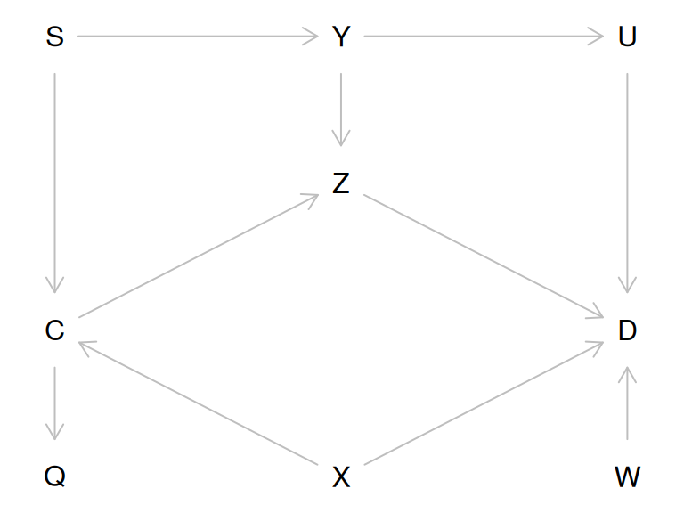
Let’s look at all possible paths from \(C\) to \(D\):
## $paths
## [1] "C -> Z -> D"           "C -> Z <- Y -> U -> D" "C <- S -> Y -> U -> D"
## [4] "C <- S -> Y -> Z -> D" "C <- X -> D"
##
## $open
## [1]  TRUE FALSE  TRUE  TRUE  TRUE
As you see, one path contains a collider and is therefore a closed path and the others are open.
Let’s identify the minimal sets of variables needed to adjust the model for \(D\) for, to obtain an unbiased estimate of the effect of \(C\). You can specify, whether you want to estimate direct or total effect of \(C\):
## { U, X, Z }
## { X, Y, Z }## { X, Y }
## { S, X }Thus, for total effect estimation one should adjust for \(X\) and either \(Y\) or \(S\), whereas for direct effect estimation, one would also need to adjust for \(Z\).
You can verify that, these are the variables that will block all open paths from \(C\) to \(D\).
Now try to do the beer-weight exercise using dagitty:
- Create the DAG and plot it
bg <- dagitty("dag {
  SEX -> BEER -> BP
  SEX -> WEIGHT -> BP
  }")
coordinates(bg) <-
  list(
    x = c(BEER = 1, SEX = 2, BP = 2, WEIGHT = 3),
    y = c(SEX = 1, BEER = 2, WEIGHT = 2, BP = 3)
  )
plot(bg)
- What are the paths from WEIGHT to BEER?
## $paths
## [1] "BEER -> BP <- WEIGHT"  "BEER <- SEX -> WEIGHT"
##
## $open
## [1] FALSE TRUE- Will you get the same recommendation for the adjustment variable selection as you found before?
Solution.
## { SEX }Effect of beer on blood pressure?
Let’s first add the effect of beer on weight to the DAG, then look at the recommended adjustment sets.
bg2 <- dagitty("dag {
  SEX -> BEER -> BP
  SEX -> WEIGHT -> BP
  BEER -> WEIGHT
  }")
coordinates(bg2) <-
  list(
    x = c(BEER = 1, SEX = 2, BP = 2, WEIGHT = 3),
    y = c(SEX = 1, BEER = 2, WEIGHT = 2, BP = 3)
  )
plot(bg2)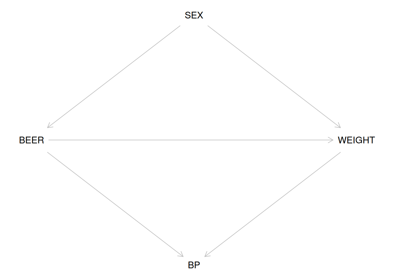
## { WEIGHT }## { SEX }Conclusions:
- To identify the direct effect, adjust for weight
- To identify the total effect, adjust for sex
9.3 Identifying the true DAG for the data
The following code creates three DAGs
par(mfrow=c(1,3))
g1 <- dagitty("dag {
    U -> Z -> Y
    U -> X
    W -> Y
    Q -> W -> X
    Q -> Y
    }")
g2 <- dagitty("dag {
    U -> Z -> Y -> W
    U -> X -> W
    Q -> W
    Q -> Y
    }")
g3 <- dagitty("dag {
    U -> Z -> Y
    U -> X -> W  -> Y
    Q -> W
    Q -> Y
    }")
coord <-
  list( x = c(X=1, U = 1.3, W = 2, Z = 2.3, Q = 2.7, Y=3),
        y = c(U=1,   Z=1.3, X=2, Y=2,   W=2.7,  Q=3)
  )
coordinates(g1)<-coordinates(g2)<-coordinates(g3)<-coord
plot(g1)
title("(a)")
plot(g2)
title("(b)")
plot(g3)
title("(c)")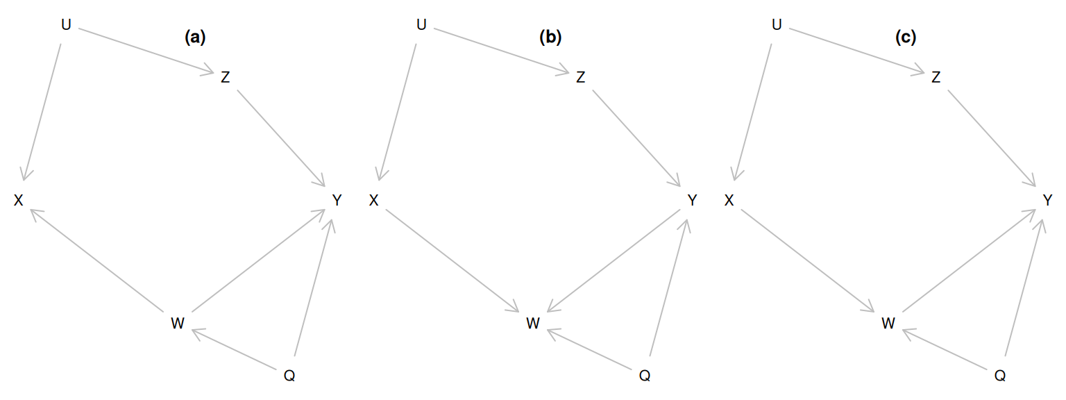
Now, the following script generates a dataset:
##        Q      W      X      Z       Y
## 1 -0.397  1.056  0.199 -0.372  -4.198
## 2  0.460  2.393 -1.647 -3.004 -10.667
## 3  0.164 -0.364  0.205 -0.852  -1.830
## 4  1.584  3.285 -9.941  2.752  -4.121
## 5  1.048  1.637  0.783 -2.047  -4.378
## 6  1.895  3.272 -3.900 -2.313  -9.871
Exercise: Using linear models, try to identify, which of the three DAGs has been used to generate the data.
Idea: If you adjust for appropriate confounders for a given DAG, you should see no effect of X on Y.
## { W, Z }
## { U, W }##
## Call:
## lm(formula = Y ~ X + W + Z, data = dat)
##
## Residuals:
## Min 1Q Median 3Q Max
## -3.9888 -0.7441 0.0096 0.7657 3.5928
##
## Coefficients:
## Estimate Std. Error t value Pr(>|t|)
## (Intercept) 0.033168 0.024551 1.351 0.177
## X -0.001691 0.014877 -0.114 0.909
## W -2.599607 0.031987 -81.270 <2e-16 ***
## Z 1.014166 0.021197 47.846 <2e-16 ***
## ---
## Signif. codes: 0 '***' 0.001 '**' 0.01 '*' 0.05 '.' 0.1 ' ' 1
##
## Residual standard error: 1.097 on 1996 degrees of freedom
## Multiple R-squared: 0.9686, Adjusted R-squared: 0.9686
## F-statistic: 2.054e+04 on 3 and 1996 DF, p-value: < 2.2e-16The DAG would be possible, if there is not effect of X.
Solution. Apparently no effect of X: this DAG “g1” (a) is possible
## { Z }
## { U }##
## Call:
## lm(formula = Y ~ X + Z, data = dat)
##
## Residuals:
## Min 1Q Median 3Q Max
## -7.480 -1.568 -0.107 1.580 8.730
##
## Coefficients:
## Estimate Std. Error t value Pr(>|t|)
## (Intercept) 0.10067 0.05092 1.977 0.0482 *
## X 1.13137 0.01077 105.040 <2e-16 ***
## Z 2.38032 0.02680 88.830 <2e-16 ***
## ---
## Signif. codes: 0 '***' 0.001 '**' 0.01 '*' 0.05 '.' 0.1 ' ' 1
##
## Residual standard error: 2.277 on 1997 degrees of freedom
## Multiple R-squared: 0.8648, Adjusted R-squared: 0.8647
## F-statistic: 6387 on 2 and 1997 DF, p-value: < 2.2e-16Solution. A clear effect of X: this DAG “g2” (b) is not likely
## { Q, W, Z }
## { Q, U, W }##
## Call:
## lm(formula = Y ~ X + Q + W + Z, data = dat)
##
## Residuals:
## Min 1Q Median 3Q Max
## -3.7210 -0.6425 0.0031 0.6596 3.1985
##
## Coefficients:
## Estimate Std. Error t value Pr(>|t|)
## (Intercept) 0.019576 0.022168 0.883 0.377
## X -0.006038 0.013429 -0.450 0.653
## Q 1.071881 0.050242 21.335 <2e-16 ***
## W -3.033392 0.035312 -85.903 <2e-16 ***
## Z 1.003544 0.019138 52.437 <2e-16 ***
## ---
## Signif. codes: 0 '***' 0.001 '**' 0.01 '*' 0.05 '.' 0.1 ' ' 1
##
## Residual standard error: 0.9903 on 1995 degrees of freedom
## Multiple R-squared: 0.9745, Adjusted R-squared: 0.9744
## F-statistic: 1.902e+04 on 4 and 1995 DF, p-value: < 2.2e-16You have probably seen that one of the three DAGs is definitely wrong for the data. But what about two others? If you are unsure, try to think of a different model to fit - you may use another dependent variable than Y (see solutions for one option).
If you have made your decision, you may check the script ‘gendata.r’ to see, whether your guess was right.
Solution. Apparently no effect of X: this DAG “g3” (c) is possible
Problem: Both (a) and (c) are possible, based on the fitted models. How to make a distinction?
Answer 1: If (c)/g3 was the correct model, we could have seen a non-zero effect of X in the first model (based on g1) that was adjusted for Z and W, but not for Q. The fact that we did not see it, rather suggests (a) as the correct model. However - absence of statistical significance is not equivalent to absence of an effect.
Another idea: Let’s find something else that helps to distinguish between (a) and (c) - can we clearly reject one of the two? For instance, let’s consider the effect of Q on X. In (a)/g1, Q has an indirect effect on X via W, thus the unadjusted model would show an effect, but not the adjusted model. In (c)/g3, W is a collider – thus an unadjusted analysis should show no effect (but adjusting for W might lead to a non-zero parameter estimate). In both cases, the other paths contain a collider (Y). Let’s confirm that with dagitty and fit the appropriate models.
## { W }## {}##
## Call:
## lm(formula = Q ~ X, data = dat)
##
## Residuals:
## Min 1Q Median 3Q Max
## -2.09466 -0.43545 -0.00958 0.44366 2.19727
##
## Coefficients:
## Estimate Std. Error t value Pr(>|t|)
## (Intercept) 0.006720 0.014824 0.453 0.65
## X -0.131401 0.002712 -48.458 <2e-16 ***
## ---
## Signif. codes: 0 '***' 0.001 '**' 0.01 '*' 0.05 '.' 0.1 ' ' 1
##
## Residual standard error: 0.663 on 1998 degrees of freedom
## Multiple R-squared: 0.5403, Adjusted R-squared: 0.5401
## F-statistic: 2348 on 1 and 1998 DF, p-value: < 2.2e-16##
## Call:
## lm(formula = Q ~ X + W, data = dat)
##
## Residuals:
## Min 1Q Median 3Q Max
## -1.65026 -0.29964 -0.00512 0.31558 1.40692
##
## Coefficients:
## Estimate Std. Error t value Pr(>|t|)
## (Intercept) 0.012290 0.009867 1.246 0.213
## X -0.001856 0.003152 -0.589 0.556
## W 0.392835 0.007836 50.134 <2e-16 ***
## ---
## Signif. codes: 0 '***' 0.001 '**' 0.01 '*' 0.05 '.' 0.1 ' ' 1
##
## Residual standard error: 0.4412 on 1997 degrees of freedom
## Multiple R-squared: 0.7965, Adjusted R-squared: 0.7963
## F-statistic: 3907 on 2 and 1997 DF, p-value: < 2.2e-16Conclusion: unadjusted model shows a clear effect, disappearing after adjustment for W. Thus we can reject (c)/g3 and conclude that (a)/g1 is the correct model.
If you have made your decision, you may check the script ‘gendata.r’ to see, whether your guess was right.
Solution.
### The contents of gendat.r
###
set.seed(202406)
n=2000
U = rnorm(n)
dat = data.frame(Q = rnorm(n))
dat$W = 2*dat$Q+rnorm(n)        #  Q -> W
dat$X = -2*dat$W +3*U+ rnorm(n) #  W -> X,  U -> X
dat$Z = -2*U+rnorm(n)           #  U -> Z
dat$Y = dat$Z-3*dat$W+dat$Q+rnorm(n) # Z -> Y, W -> Y, Q -> Y
rm(U)
dat<- round(dat,3)
Correct answer: the data was generated to follow DAG g1 (a).
9.4 Instrumental variables estimation: Mendelian randomization
Suppose you want to estimate the effect of Body Mass Index (BMI) on blood glucose level (associated with the risk of diabetes). Let’s conduct a simulation study to verify that when the exposure-outcome association is confounded, but there is a valid instrument (genotype), one obtains an unbiased estimate of the causal effect.
- Start by generating the genotype variable as Binomial(2,p), with \(p=0.2\) (and look at the resulting genotype frequencies):
##
##    0    1    2
## 6394 3243 363- Also generate the confounder variable U
- Generate a continuous (normally distributed) exposure variable \(BMI\) so that it depends on \(G\) and \(U\). Check with linear regression, whether there is enough power to get significant parameter estimates.
For instance:
- Finally generate \(Y\) (“Blood glucose level”) so that it depends on \(BMI\) and \(U\) (but not on \(G\)).
- Verify, that simple regression model for \(Y\), with \(BMI\) as a covariate, results in a biased estimate of the causal effect (parameter estimate is different from what was generated)
## Estimate StdErr z P 2.5% 97.5%
## (Intercept) 17.814562 0.097792556 182.1668 0 17.6228919 18.0062316
## BMI -0.486091 0.003850138 -126.2529 0 -0.4936372 -0.4785449How different is the estimate from 0.1?
- Estimate a regression model for \(Y\) with two covariates, \(G\) and \(BMI\). Do you see a significant effect of \(G\)? Could you explain analytically, why one may see a significant parameter estimate for \(G\) there?
## Estimate StdErr z P 2.5%
## (Intercept) 18.0909026 0.094546402 191.34417 0.000000e+00 17.9055950
## G 0.4322114 0.015159003 28.51186 8.349696e-179 0.4025003
## BMI -0.5037944 0.003754425 -134.18684 0.000000e+00 -0.5111529
## 97.5%
## (Intercept) 18.2762101
## G 0.4619225
## BMI -0.4964359- Find an IV (instrumental variables) estimate, using G as an instrument, by following the algorithm in the lecture notes (use two linear models and find a ratio of the parameter estimates). Does the estimate get closer to the generated effect size?
## Estimate StdErr z P 2.5% 97.5%
## (Intercept) 25.0344094 0.02728767 917.4255 0.000000e+00 24.9809266 25.087892
## G 0.6677507 0.03982435 16.7674 4.226261e-63 0.5896964 0.745805bgx <- mgx$coef[2] # save the 2nd coefficient (coef of G)
mgy <- lm(Y ~ G, data = mrdat)
ci.lin(mgy)## Estimate StdErr z P 2.5% 97.5%
## (Intercept) 5.47870698 0.01714404 319.569267 0.0000000000 5.44510528 5.5123087
## G 0.09580235 0.02502046 3.828961 0.0001286856 0.04676316 0.1448416## G
## 0.1434702- A proper simulation study would require the analysis to be run several times, to see the extent of variability in the parameter estimates. A simple way to do it here would be using a
for-loop. Modify the code as follows (exactly the same commands as executed so far, adding a few lines of code to the beginning and to the end):
n <- 10000
# initializing simulations:
# 30 simulations (change it, if you want more):
nsim <- 30
mr <- rep(NA, nsim) # empty vector for the outcome parameters
for (i in 1:nsim) { # start the loop
## Exactly the same commands as before:
mrdat <- data.frame(G = rbinom(n, 2, 0.2))
mrdat$U <- rnorm(n)
mrdat$BMI <-
with(mrdat, 25 + 0.7 * G + 2 * U + rnorm(n))
mrdat$Y <-
  with(mrdat, 3 + 0.1 * BMI - 1.5 * U + rnorm(n, 0, 0.5))
mgx <- lm(BMI ~ G, data = mrdat)
bgx <- mgx$coef[2]
mgy <- lm(Y ~ G, data = mrdat)
bgy <- mgy$coef[2]
# Save the i'th parameter estimate:
mr[i] <- bgy / bgx
} # end the loopNow look at the distribution of the parameter estimate:
##    Min. 1st Qu.  Median    Mean 3rd Qu.    Max.
## 0.03929 0.07114 0.09158 0.09942 0.12628 0.18344- (optional) Change the code of simulations so that the assumptions are violated: add a weak direct effect of the genotype G to the equation that generates \(Y\):
Repeat the simulation study to see, what is the bias in the average estimated causal effect of \(BMI\) on \(Y\).
- (optional) Using library
semand functiontsls, one can obtain a two-stage least squares estimate for the
causal effect and also the proper standard error. Do you get the same estimate as before?
if (!("sem" %in% installed.packages())) install.packages("sem")
library(sem)
summary(tsls(Y ~ BMI, ~G, data = mrdat))
##
## 2SLS Estimates
##
## Model Formula: Y ~ BMI
##
## Instruments: ~G
##
## Residuals:
## Min. 1st Qu. Median Mean 3rd Qu. Max.
## -6.67516 -1.12096 0.01737 0.00000 1.14845 6.30438
##
## Estimate Std. Error t value Pr(>|t|)
## (Intercept) 1.82986792 1.05930298 1.72743 0.08412200 .
## BMI 0.14814836 0.04198705 3.52843 0.00041991 ***
## ---
## Signif. codes: 0 '***' 0.001 '**' 0.01 '*' 0.05 '.' 0.1 ' ' 1
##
## Residual standard error: 1.6870674 on 9998 degrees of freedom(There are also several other R packages for IV estimation and Mendelian Randomization (MendelianRandomization for instance))
9.5 Why are simulation exercises useful for causal inference?
If we simulate the data, we know the data-generating mechanism and the true causal effects. So this is a way to check, whether an analysis approach will lead to estimates that correspond to what is generated. One could expect to see similar phenomena in real data analysis, if the data-generation mechanism is similar to what was used in simulations.