Chapter 12 Time-splitting, time-scales and SMR
This exercise is about mortaity among Danish Diabetes patients. It is
based on the dataset DMlate, a random sample of 10,000
patients from the Danish Diabetes Register (scrambeled dates), all
with date of diagnosis after 1994.
Start by loading the relevant packages:
Loading required package: nlmeThis is mgcv 1.9-1. For overview type 'help("mgcv-package")'.── Attaching core tidyverse packages ────────────────────────────────── tidyverse 2.0.0 ──
✔ dplyr 1.1.4 ✔ readr 2.1.5
✔ forcats 1.0.0 ✔ stringr 1.5.1
✔ ggplot2 3.5.1 ✔ tibble 3.2.1
✔ lubridate 1.9.3 ✔ tidyr 1.3.1
✔ purrr 1.0.2 ── Conflicts ──────────────────────────────────────────────────── tidyverse_conflicts() ──
✖ dplyr::collapse() masks nlme::collapse()
✖ dplyr::filter() masks stats::filter()
✖ lubridate::is.Date() masks popEpi::is.Date()
✖ dplyr::lag() masks stats::lag()
ℹ Use the conflicted package (<http://conflicted.r-lib.org/>) to force all conflicts to become errorsThen load the data and take a look at the data:
'data.frame':   10000 obs. of  7 variables:
 $ sex  : Factor w/ 2 levels "M","F": 2 1 2 2 1 2 1 1 2 1 ...
 $ dobth: num  1940 1939 1918 1965 1933 ...
 $ dodm : num  1999 2003 2005 2009 2009 ...
 $ dodth: num  NA NA NA NA NA ...
 $ dooad: num  NA 2007 NA NA NA ...
 $ doins: num  NA NA NA NA NA NA NA NA NA NA ...
 $ dox  : num  2010 2010 2010 2010 2010 ...
You can get a more detailed explanation of the data by referring to the help page:
Set up the dataset as a
Lexisobject with age, calendar time and duration of diabetes as timescales, and date of death as event. Make sure that you know what each of the arguments toLexismean:LL <- Lexis(entry = list(A = dodm - dobth, P = dodm, dur = 0), exit = list(P = dox), exit.status = factor(!is.na(dodth), labels = c("Alive", "Dead")), data = DMlate)NOTE: entry.status has been set to "Alive" for all. NOTE: Dropping 4 rows with duration of follow up < tolTake a look at the first few lines of the resulting dataset, for example using
head().Get an overview of the mortality by using
stat.tableto tabulate no. deaths, person-years (lex.dur) and the crude mortality rate by sex. Try:stat.table(sex, list(D = sum(lex.Xst == "Dead"), Y = sum(lex.dur), rate = ratio(lex.Xst == "Dead", lex.dur, 1000)), margins = TRUE, data = LL)--------------------------------- sex D Y rate --------------------------------- M 1343.00 27614.21 48.63 F 1156.00 26659.05 43.36 Total 2499.00 54273.27 46.04 ---------------------------------# stat.table is more versatile than xtabs: xtabs(cbind(D = lex.Xst == "Dead", Y = lex.dur) ~ sex, data = LL)sex D Y M 1343.00 27614.21 F 1156.00 26659.05If we want to assess how mortality depends on age, calendar time and duration or how it relates to population mortality, we should in principle split the follow-up along all three time scales. In practice it is sufficient to split it along one of the time-scales and then use the value of each of the time-scales at the left endpoint of the intervals.
Use
splitLexis(orsplitMultifrom thepopEpipackage) to split the follow-up along the age-axis in sutiable intervals (here set to 1/2 year, but really immaterial as long as it is small):Transitions: To From Alive Dead Records: Events: Risk time: Persons: Alive 115974 2499 118473 2499 54273.27 9996How many records are now in the dataset? How many person-years? Compare to the original
Lexis-dataset.
12.1 Age-specific mortality
Now estimate age-specific mortality curves for men and women separately, using splines as implemented in
gam. We usek = 20to be sure to catch any irregularities by age.r.m <- mgcv::gam(cbind(lex.Xst == "Dead", lex.dur) ~ s(A, k = 20), family = poisreg, data = subset(SL, sex == "M"))Make sure you understand all the components on this modeling statement. Fit the same model for women.
There is a convenient wrapper for this, exploiting the
Lexisstructure of data, but which does not have an updatemgcv::gam Poisson analysis of Lexis object subset(SL, sex == "M") with log link: Rates for the transition: Alive->Deadmgcv::gam Poisson analysis of Lexis object subset(SL, sex == "F") with log link: Rates for the transition: Alive->DeadNow, extract the estimated rates by using the wrapper function
ci.predthat computes predicted rates and confidence limits for these.glm.Lexisandgam.Lexisuse thepoisregfamily that will return the rates in the (inverse) units in which the person-years were given; that is the units in whichlex.duris recorded.nd <- data.frame(A = seq(20, 90, 0.5)) p.m <- ci.pred(r.m, newdata = nd) p.f <- ci.pred(r.f, newdata = nd) str(p.m)num [1:141, 1:3] 0.00132 0.00137 0.00142 0.00147 0.00152 ... - attr(*, "dimnames")=List of 2 ..$ : chr [1:141] "1" "2" "3" "4" ... ..$ : chr [1:3] "Estimate" "2.5%" "97.5%"Plot the predicted rates for men and women together - using for example
matplotormatshade.par(mar = c(3.5,3.5,1,1), mgp = c(3,1,0) / 1.6, las = 1, bty = "n", lend = "butt") matplot(nd$A, cbind(p.m, p.f) * 1000, type = "l", col = rep(c("blue", "red"), each = 3), lwd = c(3, 1, 1), lty = 1, log = "y", yaxt = "n", xlab = "Age", ylab = "Mortality per 1000 PY") axis(side = 2, at = ll <- outer( c(5, 10, 20), -1:1, function(x,y) x * 10^y), labels = ll)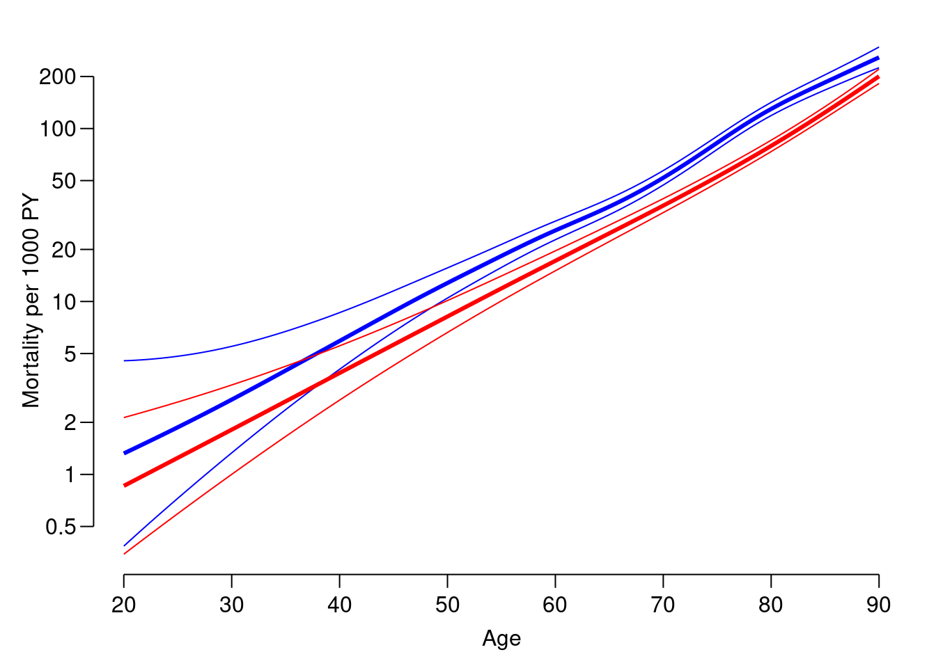
Further time scales: period and duration
We now want to model the mortality rates among diabetes patients also including current date and duration of diabetes, using penalized splines. Use the argument
bs = "cr"tos()to get cubic splines instead of thin plate ("tp") splines which is the default.As before specify the model exploiting the
Lexisclass of the dataset, try:Mcr <- gam.Lexis(subset(SL, sex == "M"), ~ s(A, bs = "cr", k = 10) + s(P, bs = "cr", k = 10) + s(dur, bs = "cr", k = 10))mgcv::gam Poisson analysis of Lexis object subset(SL, sex == "M") with log link: Rates for the transition: Alive->DeadFamily: poisson Link function: log Formula: cbind(trt(Lx$lex.Cst, Lx$lex.Xst) %in% trnam, Lx$lex.dur) ~ s(A, bs = "cr", k = 10) + s(P, bs = "cr", k = 10) + s(dur, bs = "cr", k = 10) Parametric coefficients: Estimate Std. Error z value Pr(>|z|) (Intercept) -3.54074 0.04938 -71.7 <2e-16 Approximate significance of smooth terms: edf Ref.df Chi.sq p-value s(A) 3.645 4.517 1013.20 < 2e-16 s(P) 1.024 1.048 17.58 3.48e-05 s(dur) 7.586 8.384 74.46 < 2e-16 R-sq.(adj) = 0.00333 Deviance explained = 9.87% UBRE = -0.8054 Scale est. = 1 n = 60347Fit the same model for women as well. Are the models reasonably fitting?
Fcr <- gam.Lexis(subset(SL, sex == "F"),
                 ~ s(A, bs = "cr", k = 10) +
                   s(P, bs = "cr", k = 10) +
                 s(dur, bs = "cr", k = 10))
mgcv::gam Poisson analysis of Lexis object subset(SL, sex == "F") with log link: Rates for the transition: Alive->DeadFamily: poisson Link function: log Formula: cbind(trt(Lx$lex.Cst, Lx$lex.Xst) %in% trnam, Lx$lex.dur) ~ s(A, bs = "cr", k = 10) + s(P, bs = "cr", k = 10) + s(dur, bs = "cr", k = 10) Parametric coefficients: Estimate Std. Error z value Pr(>|z|) (Intercept) -3.78483 0.05808 -65.17 <2e-16 Approximate significance of smooth terms: edf Ref.df Chi.sq p-value s(A) 2.667 3.366 988.49 < 2e-16 s(P) 1.904 2.391 20.08 0.000136 s(dur) 5.973 6.972 38.98 < 2e-16 R-sq.(adj) = 0.00417 Deviance explained = 11.1% UBRE = -0.82405 Scale est. = 1 n = 58126Plot the estimated effects, using the default plot method for
gamobjects. Remember that there are three effects estimated, so it is useful set up a multi-panel display, and for the sake of comparability to set ylim to the same for men and women: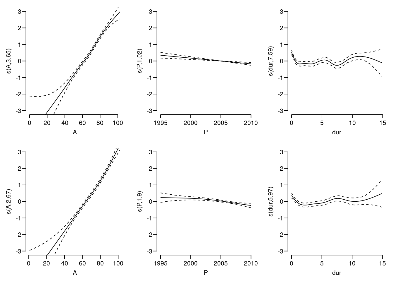
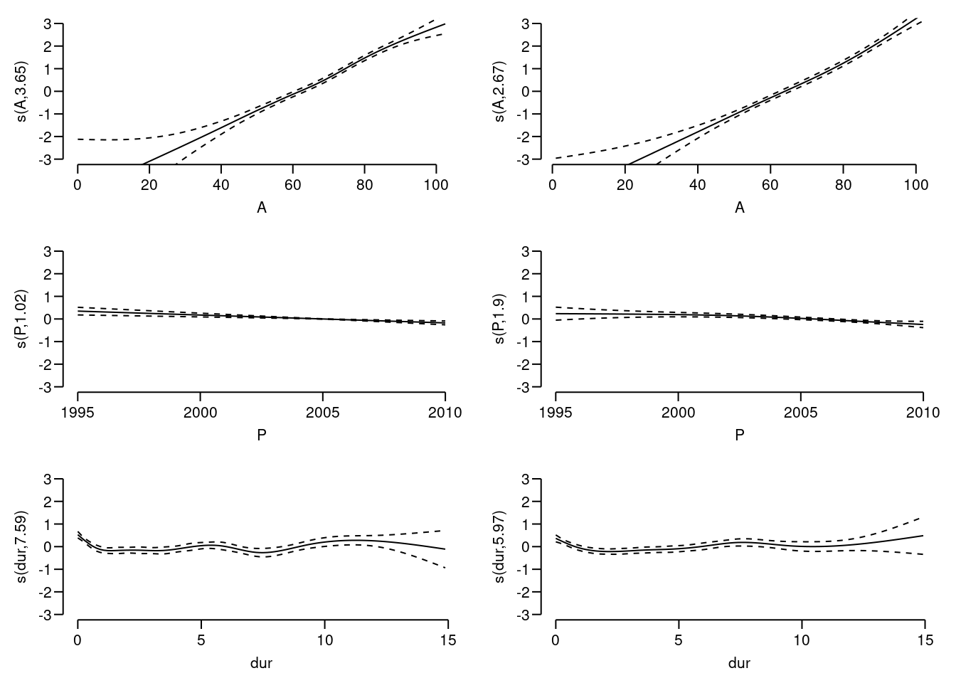 What is the absolute scale for these effects?
Compare the fit of the naive model with just age and the three-factor models, using
anova, e.g.:Analysis of Deviance Table Model 1: cbind(trt(Lx$lex.Cst, Lx$lex.Xst) %in% trnam, Lx$lex.dur) ~ s(A, bs = "cr", k = 10) + s(P, bs = "cr", k = 10) + s(dur, bs = "cr", k = 10) Model 2: cbind(trt(Lx$lex.Cst, Lx$lex.Xst) %in% trnam, Lx$lex.dur) ~ s(A, k = 20) Resid. Df Resid. Dev Df Deviance Pr(>Chi) 1 60332 11717 2 60340 11812 -7.9484 -95.094 < 2.2e-16What do you conclude?
The model we fitted has three time-scales: current age, current date and current duration of diabetes, so the effects that we report are not immediately interpretable, as they are (as in any kind of multiple regressions) to be interpreted as all else equal which they are not, as the three time scales advance simultaneously at the same pace.
The reporting would therefore more naturally be on the mortality scale as a function of age, but showing the mortality for persons diagnosed in different ages, using separate displays for separate years of diagnosis. This is most easily done using the
ci.predfunction with thenewdata =argument. So a person diagnosed in age 50 in 1995 will have a mortality measured in cases per 1000 PY as:pts <- seq(0, 12, 1/4) nd <- data.frame(A = 50 + pts, P = 1995 + pts, dur = pts) m.pr <- ci.pred(Mcr, newdata = nd)Note that because we used
gam.Lexiswhich uses thepoisregfamily we need not specifylex.duras a variable in the prediction data framend. Predictions will be rates in the same units aslex.dur(well, the inverse).Now take a look at the result from the
ci.predstatement and construct prediction of mortality for men and women diagnosed in a range of ages, say 50, 60, 70, and plot these together in the same graph:From figure it seems that the duration effect is over-modeled, so refit constraining the d.f. to 5:
Mcr <- gam.Lexis(subset(SL, sex == "M"),
                 ~ s(A, bs = "cr", k = 10) +
                   s(P, bs = "cr", k = 10) +
                 s(dur, bs = "cr", k = 5))
mgcv::gam Poisson analysis of Lexis object subset(SL, sex == "M") with log link: Rates for the transition: Alive->DeadFcr <- gam.Lexis(subset(SL, sex == "F"), ~ s(A, bs = "cr", k = 10) + s(P, bs = "cr", k = 10) + s(dur, bs = "cr", k = 5))mgcv::gam Poisson analysis of Lexis object subset(SL, sex == "F") with log link: Rates for the transition: Alive->DeadPlot the estimated rates from the revised models. What do you conclude from the plots?
12.2 SMR
The SMR is the Standardized Mortality Ratio, which is the mortality rate-ratio between the diabetes patients and the general population. In real studies we would subtract the deaths and the person-years among the diabetes patients from those of the general population, but since we do not have access to these, we make the comparison to the general population at large, i.e. also including the diabetes patients.
So we now want to include the population mortality rates as a fixed variable in the split dataset; for each record in the split dataset we attach the value of the population mortality for the relevant sex, and and calendar time.
This can be achieved in two ways: Either we just use the current split of follow-up time and allocate the population mortality rates for some suitably chosen (mid-)point of the follow-up in each, or we make a second split by date, so that follow-up in the diabetes patients is in the same classification of age and data as the population mortality table.
We will use the former approach, using the dataset split in 6 month intervals, and then include as an extra variable the population mortality as available from the data set
M.dk.First create the variables in the diabetes dataset that we need for matching with the population mortality data, that is sex and age and date at the midpoint of each of the intervals (or rather at a point 3 months after the left endpoint of the interval; recall we split the follow-up in 6 month intervals).
We need to have variables of the same type when we merge, so we must transform the sex variable in
M.dkto a factor, and must for each follow-up interval in theSLdata have an age and a period variable that can be used in merging with the population data.Classes 'Lexis' and 'data.frame': 118473 obs. of 14 variables: $ lex.id : int 1 1 1 1 1 1 1 1 1 1 ... $ A : num 58.7 59 59.5 60 60.5 ... $ P : num 1999 1999 2000 2000 2001 ... $ dur : num 0 0.339 0.839 1.339 1.839 ... $ lex.dur: num 0.339 0.5 0.5 0.5 0.5 ... $ lex.Cst: Factor w/ 2 levels "Alive","Dead": 1 1 1 1 1 1 1 1 1 1 ... $ lex.Xst: Factor w/ 2 levels "Alive","Dead": 1 1 1 1 1 1 1 1 1 1 ... $ sex : Factor w/ 2 levels "M","F": 2 2 2 2 2 2 2 2 2 2 ... $ dobth : num 1940 1940 1940 1940 1940 ... $ dodm : num 1999 1999 1999 1999 1999 ... $ dodth : num NA NA NA NA NA NA NA NA NA NA ... $ dooad : num NA NA NA NA NA NA NA NA NA NA ... $ doins : num NA NA NA NA NA NA NA NA NA NA ... $ dox : num 2010 2010 2010 2010 2010 ... - attr(*, "breaks")=List of 3 ..$ A : num [1:251] 0 0.5 1 1.5 2 2.5 3 3.5 4 4.5 ... ..$ P : NULL ..$ dur: NULL - attr(*, "time.scales")= chr [1:3] "A" "P" "dur" - attr(*, "time.since")= chr [1:3] "" "" ""'data.frame': 7800 obs. of 6 variables: $ A : num 0 0 0 0 0 0 0 0 0 0 ... $ sex : num 1 2 1 2 1 2 1 2 1 2 ... $ P : num 1974 1974 1975 1975 1976 ... $ D : num 459 303 435 311 405 258 332 205 312 233 ... $ Y : num 35963 34383 36099 34652 34965 ... $ rate: num 12.76 8.81 12.05 8.97 11.58 ... - attr(*, "Contents")= chr "Number of deaths and risk time in Denmark"'data.frame': 7800 obs. of 8 variables: $ A : num 0 0 0 0 0 0 0 0 0 0 ... $ sex : Factor w/ 2 levels "M","F": 1 2 1 2 1 2 1 2 1 2 ... $ P : num 1974 1974 1975 1975 1976 ... $ D : num 459 303 435 311 405 258 332 205 312 233 ... $ Y : num 35963 34383 36099 34652 34965 ... $ rate: num 12.76 8.81 12.05 8.97 11.58 ... $ Am : num 0 0 0 0 0 0 0 0 0 0 ... $ Pm : num 1974 1974 1975 1975 1976 ...Then match the rates from
M.dkintoSL;sex,AmandPmare the common variables, and therefore the match is on these variables:[1] 118473 16[1] 118454 17This merge (remember to
?merge!) only takes rows that have information from both datasets, hence the slightly fewer rows inSLrthan inSL.- Compute the expected number of deaths as the person-time
multiplied (
lex.dur) by the corresponding population rate, and put it in a new variable,E, say (Expected). Usestat.tableto make a table of observed, expected and the ratio (SMR) by age (suitably grouped, look forcut) and sex.
- Compute the expected number of deaths as the person-time
multiplied (
Fit a poisson model with sex as the explanatory variable and log-expected as offset to derive the SMR (and c.i.). Some of the population mortality rates are 0, so you need to exclude those records from the analysis.
msmr <- glm((lex.Xst == "Dead") ~ sex - 1,
            offset = log(E),
            family = poisson,
              data = subset(SLr, E > 0))
ci.exp(msmr)
exp(Est.) 2.5% 97.5% sexM 1.685699 1.597881 1.778344 sexF 1.541922 1.455442 1.633540Do you recognize the numbers?
- The same model can be fitted a bit simpler by the
poisregfamily, try:
msmr <- glm(cbind(lex.Xst == "Dead", E) ~ sex - 1,
            family = poisreg,
              data = subset(SLr, E > 0))
ci.exp(msmr)
exp(Est.) 2.5% 97.5% sexM 1.685699 1.597881 1.778344 sexF 1.541922 1.455441 1.633541We can assess the ratios of SMRs between men and women by using the
ctr.matargument which should be a matrix:[,1] [,2] M 1 0 W 0 1 M/F 1 -1exp(Est.) 2.5% 97.5% M 1.69 1.60 1.78 W 1.54 1.46 1.63 M/F 1.09 1.01 1.18What do you conclude about the mortality rates among men and women?
- The same model can be fitted a bit simpler by the
12.3 SMR modeling
Now model the SMR using age and date of diagnosis and diabetes duration as explanatory variables, including the expected-number instead of the person-years, using separate models for men and women.
Note that you cannot use
gam.Lexisfrom the code you used for fitting models for the rates, you need to usegamwith thepoisregfamily. And remember to exclude those units where no deaths in the population occur (that is where the population mortality rate is 0).Msmr <- gam(cbind(lex.Xst == "Dead", E) ~ s( A, bs = "cr", k = 5) + s( P, bs = "cr", k = 5) + s(dur, bs = "cr", k = 5), family = poisreg, data = subset(SLr, E > 0 & sex == "M")) ci.exp(Msmr)exp(Est.) 2.5% 97.5% (Intercept) 2.1667053 2.0001046 2.3471833 s(A).1 0.5960527 0.5181962 0.6856068 s(A).2 0.8927331 0.8650901 0.9212594 s(A).3 0.3663506 0.2818154 0.4762435 s(A).4 0.4587803 0.3763049 0.5593320 s(P).1 0.9893048 0.9732835 1.0055898 s(P).2 0.9608720 0.9085181 1.0162428 s(P).3 0.9027294 0.7825209 1.0414040 s(P).4 0.9173557 0.8132938 1.0347323 s(dur).1 0.6581828 0.5769629 0.7508362 s(dur).2 0.8446645 0.7613599 0.9370838 s(dur).3 0.7830215 0.6916313 0.8864877 s(dur).4 1.8176744 1.1041338 2.9923368Plot the estimated smooth effects for both men and women using e.g.
plot.gam. What do you see?Plot the predicted SMRs from the models for men and women diagnosed in ages 50, 60 and 70 as you did for the rates. What do you see?
par(mfrow = c(1,1))
n50 <- nd
n60 <- mutate(n50, A = A + 10)
n70 <- mutate(n50, A = A + 20)
head(n70)
A P dur 1 70.00 1995.00 0.00 2 70.25 1995.25 0.25 3 70.50 1995.50 0.50 4 70.75 1995.75 0.75 5 71.00 1996.00 1.00 6 71.25 1996.25 1.25matshade(n50$A, cbind(ci.pred(Msmr, n50), ci.pred(Fsmr, n50)), plot = TRUE, col = c("blue", "red"), lwd = 3, ylim = c(0.5, 5), log = "y", xlim = c(50, 80)) matshade(n60$A, cbind(ci.pred(Msmr, n60), ci.pred(Fsmr, n60)), col = c("blue", "red"), lwd = 3) matshade(n70$A, cbind(ci.pred(Msmr, n70), ci.pred(Fsmr, n70)), col = c("blue", "red"), lwd = 3) abline(h = 1) abline(v = 50 + 0:5, lty = 3, col = "gray")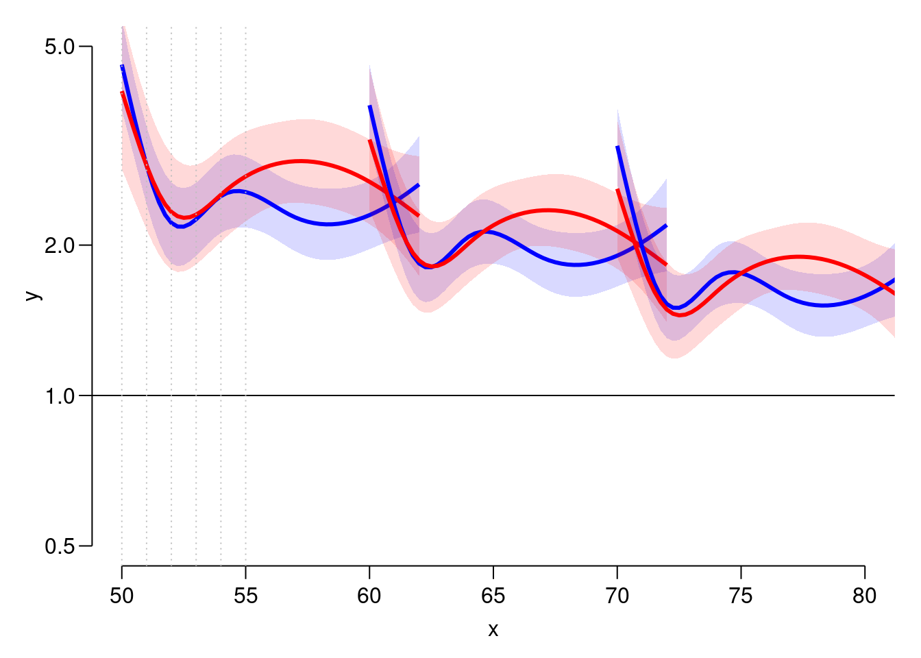 Describe the shapes of the curves. What aspects of the shapes are
induced by the model ?
Describe the shapes of the curves. What aspects of the shapes are
induced by the model ?Try to simplify the model to one with a simple sex effect, separate linear effects of age and date of follow-up for each sex, and a smooth effect of duration common for both sexes, giving an estimate of the change in SMR by age and calendar time.
Bsmr <- gam(cbind(lex.Xst == "Dead", E)
            ~ sex / A +
              sex / P +
              s(dur, bs = "cr", k = 5),
            family = poisreg,
              data = subset(SLr, E > 0))
round(ci.exp(Bsmr)[-1,], 3)
exp(Est.) 2.5% 97.5% sexF 52149.525 0.000 2.375788e+23 sexM:A 0.981 0.977 9.860000e-01 sexF:A 0.980 0.975 9.860000e-01 sexM:P 0.987 0.972 1.002000e+00 sexF:P 0.981 0.965 9.980000e-01 s(dur).1 0.663 0.601 7.320000e-01 s(dur).2 0.861 0.795 9.310000e-01 s(dur).3 0.885 0.805 9.740000e-01 s(dur).4 1.412 0.945 2.111000e+00How much does SMR change by each year of age? And by each calendar year?
What is the meaning of the
sexFparameter?Use your previous code to plot the predicted mortality from this model too. Are the predicted SMR curves credible?
m50 <- mutate(n50, sex = "M") f50 <- mutate(n50, sex = "F") m60 <- mutate(m50, A = A + 10) f60 <- mutate(f50, A = A + 10) m70 <- mutate(m50, A = A + 20) f70 <- mutate(f50, A = A + 20) matshade(n50$A, cbind(ci.pred(Bsmr, m50), ci.pred(Bsmr, f50)), plot = TRUE, col = c("blue", "red"), lwd = 3, ylim = c(0.5, 5), log = "y", xlim = c(50, 80)) matshade(n60$A, cbind(ci.pred(Bsmr, m60), ci.pred(Bsmr, f60)), col = c("blue", "red"), lwd = 3) matshade(n70$A, cbind(ci.pred(Bsmr, m70), ci.pred(Bsmr, f70)), col = c("blue", "red"), lwd = 3) abline(h = 1) abline(h = 1:5, lty = 3, col = "gray")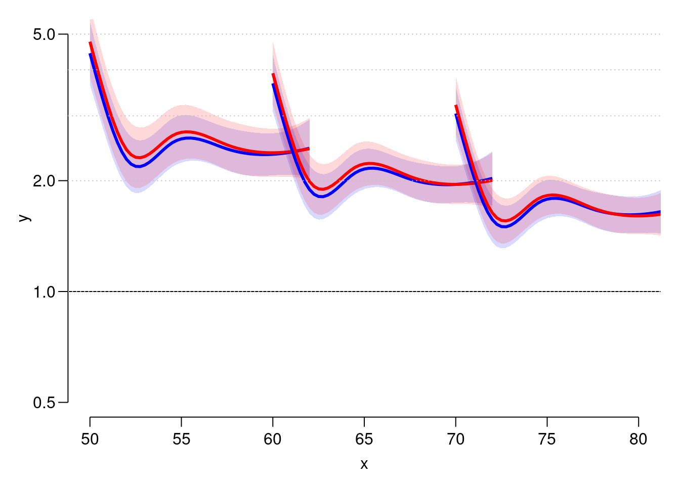 What is your conclusion about SMR for diabetes patients relative to the
general popuation?